Olivier Taché, Olivier Spalla, Antoine Thill, David Carriere, Fabienne Testard, Debassis Sen
We have developed at LIONS a series of modules grouped under the name PySAXS (like Python for SAXS). PySAXS is entirely based on Numpy and SciPy. These modules allow us to perform the different operations necessary to process the SAXS data treatment (setting in absolute scale, deconvolution, background substraction,…). Error uncertainty is taken in acount.
pySAXS is OPEN SOURCE and distributed under the CECILL licence (GPL compatible).
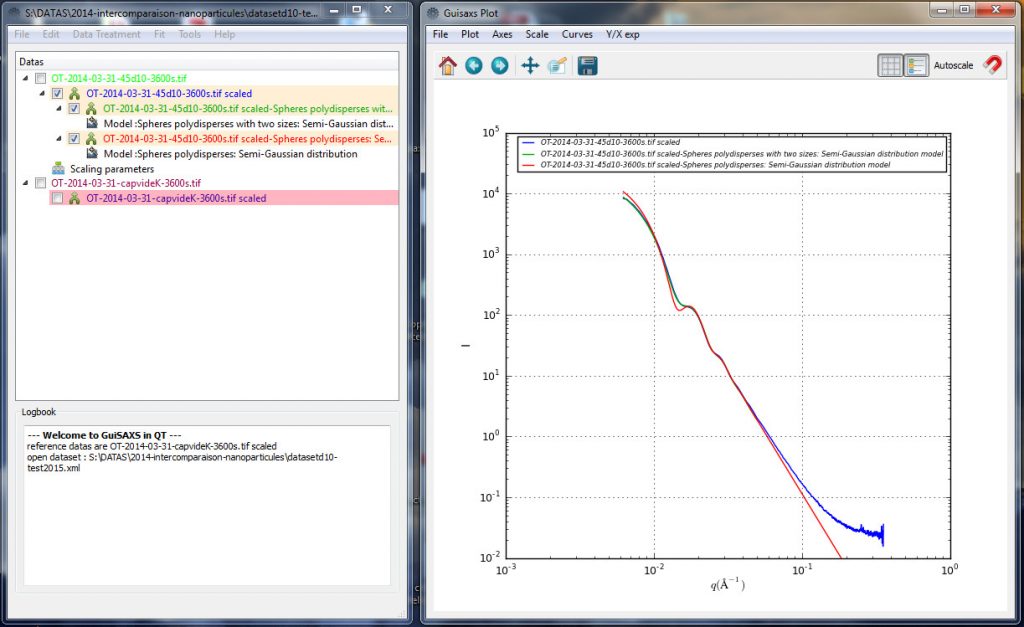
A graphic user interface (guiSAXS) developped with QT is also available.
pySAXS works with plugins systems. Some tools are developped to integrate pyFAI, MCSAS.
The software can open 1D text files from various image reduction softwares :
- chi files from fit2D,
- raw data with two columns, …,
- and data files from ou ImageJ plugins with the 3rd columns for uncertaintly.
It can simultaneously display and manipulate spectra. It’s easy to concatenate data with different abscissas, or perform mathematical operations and scaling. It is also possible to smooth or find peaks on data.
An invariant tool is also available.
DONWLOAD:
pySAS is always in constant improvement.
You can install a fresh copy with “pip install pySAXS”
Models
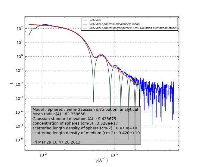
The reference models (describing different types of molecular organizations like sphere, shell or cylinder particles) are programmed by the researchers themselves.
Python language let the user to understand, verify and check the code.
Most of amplitude factor, and form factor are in the library and optimized.
Models are automatically displayed in the GUI menu. A dialog box is generated that allows overlapping data with the chosen model, to vary the settings and launch a minimization using least-square algorithm.
Already programmed models :
- Guinier
- Porod with curvature correction
- Cube
- Porod
- Multi: Triplet of identical spheres
- Spheres poly-Gauss analytic
- Multi: Doublet of identical spheres
- Gaussian
- Parallelepiped
- Core-shell cylinder
- Capsule
- Core Shell Particle
- PearsonVII
- Mono Ellipse
- Mono Cylinder
- Multi: Tetrahedra of identical spheres
- Spheres Monodisperse
- Specific: Imogolite Single Wall Si/Ge
- Trapez
- Cylinder with six levels
Fits
Users can also use the pySAXS librairies and models in programs, with a few lines of code :
#----- fit
from pySAXS.models import PearsonVII
d=PearsonVII() #declare model
d.q=datax       #q data to model
d.Arg=[amplitude,qAtMax,width,2.0,background] #initial parameters
res=d.fit(datay) #FIT !!!
Tools
The GUI proposes also some tools :
– for calculating X-Ray contrast, or transmission, with data exported from NIST X-Ray Absorption Tables.
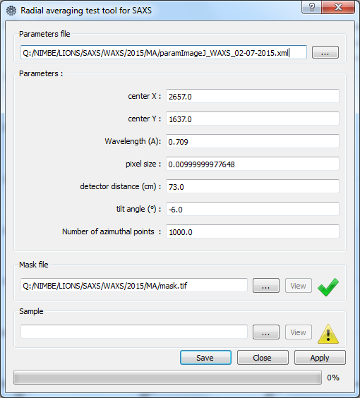
– radial averaging using pyFAI library for singles images, multiples images, and cinetic images
– MC sas integration (actually in test)
Versions and documentation
presentation :

formation SAXS pysaxs.pdf
pySAXS API documentation is here (OLD)
WARNING : for using pySAXS, you need to install Python, numpy, scipy, QT. It is recommanded to use Winpython package.
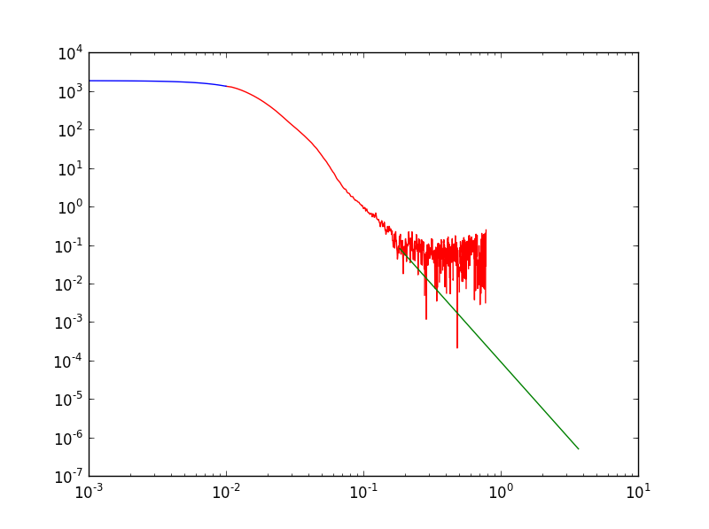
pySAXS can also be used in scripts for automatize calculation
A example for invariant
'''

example of importing data from a xml dataset

and calculate invariant with different parameters

'''

import pySAXS

from pySAXS.guisaxs.dataset import *

from pySAXS.LS import invariant

import os

import numpy

#--- import datas from file

p=os.path.dirname(pySAXS.__file__)

dataFile="dataset_examples.xml"

completeDataFile=p+os.sep+"saxsdata"+os.sep+dataFile

dt=getDataDictFromXMLFile(completeDataFile)

q=dt['JBIV61_2500super/.173'].q

i=dt['JBIV61_2500super/.173'].i
#— initialize invariant
invar=invariant.invariant(q,i,radius=30.0)
# parameters can be changed directly
invar.radius=30.0
#— or in the calculate call
invar.calculate(radius=30.0)
invar.calculate(radius=100.0)
invar.calculate(qmax=0.184,extrapolation=0.92926904607e+28) #radius=100.0
vol=invar.getVolume()
#particule radius calculation
radius=((vol*3)/(4*numpy.pi))**(1.0/3)
print “particule radius = “,radius, ” cm”
#— plot
import matplotlib.pyplot as plt
plt.plot(q,i,color=’red’)
plt.plot(invar.LowQq,invar.LowQi,color=’blue’)
plt.plot(invar.HighQq,invar.HighQi,color=’green’)
plt.yscale(‘log’)
plt.xscale(‘log’)
plt.show()
GIVES :
— Initializing invariant calculation —
I*=1329.92177419 I0=26712.2042447
I at qmin : 1329.92177419
Intensity average for last 238 positive points = 0.0777715954277
— Calculating Invariant —
qmin=0.0100000007078 qmax=0.784000039101 radius=30.0 extrapolation=2.93822700279e+30
I*=1329.92177419 I0=1370.42392784
Invariant (cm-4) = P1+P2+P3 =5.39374891641e+22
Particle Volume = 2 * PI**2 * I0 / invariant =5.01526572304e-19 cm3
— Calculating Invariant —
qmin=0.0100000007078 qmax=0.784000039101 radius=100.0 extrapolation=2.93822700279e+30
I*=1329.92177419 I0=1856.05544004
Invariant (cm-4) = P1+P2+P3 =5.39973041419e+22
Particle Volume = 2 * PI**2 * I0 / invariant =6.78498055811e-19 cm3
— Calculating Invariant —
qmin=0.0100000007078 qmax=0.184 radius=100.0 extrapolation=9.2926904607e+27
I*=1329.92177419 I0=1856.05544004
Invariant (cm-4) = P1+P2+P3 =7.34690790475e+21
Particle Volume = 2 * PI**2 * I0 / invariant =4.9867326982e-18 cm3
particule radius = 1.05984533705e-06 cm
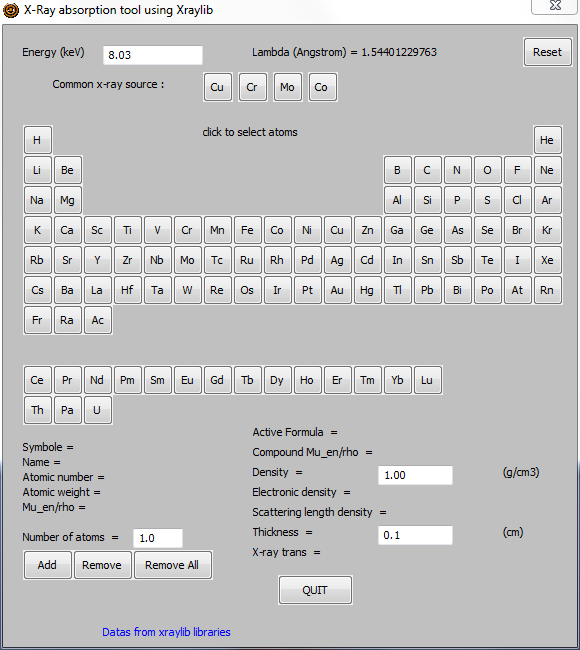
New : now pySAXS can use xraylib for absorption calculation
we change this tool for absorption calculation by using the xraylib librairies.
Xraylib is a library for X-ray matter interactions cross sections for X-ray fluorescence applications. Available HERE.
Sept 2012 : for this moment work only on windows. How to install : install xraylib with the latest windows installer.
guiSAXS is detecting if xraylib is installed and working, and propose the absorption tool.
You can use it in command line :
from pySAXS.LS import absorptionXRL
formula=”H 2 O 1″
density=1.0
thickness=0.1 #1 mm
source=’Cu’
energy=getEnergyFromSource(source)
print “energy for “,source,” : “,energy,” keV ->”,getAngstFromSource(source),’ A’
print “Calculate Mu from formula for water : “,formula
mu=getMuFormula(formula,energy)
print mu
print “X-ray transmission = “,numpy.exp(-density*mu*thickness)
print getTransmission(formula,thickness,density,energy)
print “——————–“
source=’Mo’
energy=getEnergyFromSource(source)
print “energy for “,source,” : “,energy,” keV ->”,getAngstFromSource(source),’ A’
print “Calculate Mu from formula for water : “,formula
mu=getMuFormula(formula,energy)
print mu
print “X-ray transmission = “,numpy.exp(-density*mu*thickness)
print getTransmission(formula,thickness,density,energy)
pySAXS-2.144.July2015.win-amd64.exe
